16. Neatness and legibility counts!
Format of Lab Report
1. Title
2. Objective
3. Screen capture or drawing of experiment (simulation)
4. Procedure (ok to copy and paste into notebook)
5. Data (tables)
6. Calculations and Analysis (graphs)
7. Summary of Error and Sources of Error
8. Conclusion (1 or 2 sentences)
Lab for 08-28-24
Understanding Vectors
Objective: Obtain an intuitive understanding of vectors and their addition.
Procedure
- Click on "Explore 2D" and play with the simulator until you understand how to
A) Drag vectors into the central grid from their box on the right.
B) Change the orientation of a vector by dragging its tip in a direction perpendicular to its length.
C) Change the length of a vector by dragging its tip in a direction parallel or antiparallel to its length.
D) Sum the vectors on the central grid by clicking the "Sum" box.
E) Display a vector's length, angle relative to the horizontal, and components by clicking on it.
F) Display angles of all vectors relative to the horizontal by clicking the θ box.
G) Display the lengths of all vectors by clicking the "Values" box.
- Position 2 random vectors on the simulator. Visualize their sum.
- Use simulator to add them. Repeat until your visualization matches the simulator's result.
- Use the simulator to verify the Law of Cosines by calculating the length of the sum using the Law of Cosines and comparing it to the simulator's result for 5 distinct triangles. Follow the example shown to fill out the table below.
- Are the values in the two length-of-b columns identical to 3 significant digits?
- If they are not identical, what might be the source of the error?
- Can you conclude that the it's possible to train yourself to accurately visualize the sum of two vectors? Can you conclude the the simulator is perfectly precise?
Example
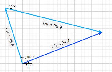
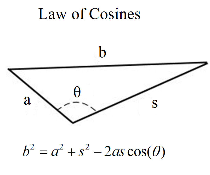
b = (16.82 + 24.72 - 2(16.8)(24.7)cos(86°))1/2 = 28.89
Error = (28.9 - 28.89)/28.9 x 100 = 0.035%
| Trial | Vector a Length | Vector s Length | Vector a Angle | Vector s Angle | (Vector a Angle) — (Vector s Angle) | Length of b (Simulator) | Length of b (Law of Cosines) | Error |
|---|---|---|---|---|---|---|---|---|
| Example | 16.8 | 24.7 | 107.4° | 21.4° | 86° | 28.9 | 28.89 | 0.035% |
| 1 | ||||||||
| 2 | ||||||||
| 3 | ||||||||
| 4 | ||||||||
| 5 |
Lab for 09-04-25
Projectile Motion
Objective: Confirm Kinematics Equations and Study Effect of Air Resistance
Procedure
- Click on the "Labs" (cannon) icon above.
- Turn air resistance OFF. Select "user choice", diameter = 0.1. For a 3 kg mass shot with an initial speed of 15 m/s, at what angle does it travel the greatest horizontal distance? [Use trial and error to find this angle by fill out the table below and graphing the results (use angle as the horizontal axis).]
Angle (degrees) Range (m) 25 30 40 45 50 55 60 - Turn air resistance ON. Answer question # 1 again.
- With air resistance OFF and mass = 1 kg, find the speed and angle required to hit a target at 18 m (± 0.3 m) in 2.8 seconds (± 0.1 second).
- With air resistance ON and mass = 1 kg, find the speed and angle required to hit a target at 18 m in 2.8 seconds.
- With air resistance ON, plot max_distance vs mass. Use the angle you obtained in step 2 and a speed of 15 m/s. Use mass values: 1, 5, 9, 13, 17, 21, 25, 29 kg.
- With air resistance OFF, repeat step 5 (using the same angle used in step 5).
Analysis
- How well does your range vs angle graph compare to the theory? [Range = Vo2sin(2θ)/(2g)].
- Does the distance traveled depend on mass, when air resistance is on?
- Does the distance traveled depend on mass, when air resistance is off?
Lab for 09-11-25
Friction
| Click to Run |
Objective: Confirm the Equations for Static and Kinetic Friction
Procedure
Part 1: Static Friction
- Open the simulation by clicking on the image above and clicking on the .jnlp file that is downloaded.
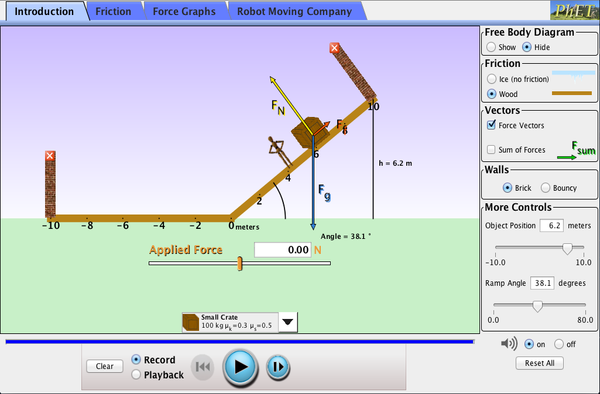
- Select the "Friction" tab. Use the following settings:
Static Friction (μs) = 0.1,
KineticFfriction (μk) = 0.1,
Object Mass = 100 kg,
Gravity = "Earth",
Ramp Angle = 0.0 degrees,
Object Position = 6 m
Friction: Wood
Walls: Brick - Create the following table.
Static Friction (μs) Ramp Angle (Observed) (deg) Ramp Angle (Theory) (deg) 0.1 0.3 0.5 0.7 1.0 1.5 2.0 - For each choice of the coefficient of static friction, slowly increase the ramp angle until the object begins to slide down. Record this "Ramp Angle (Observed)".
- Calculate arctan(μs), and enter it as the "Ramp Angle (Theory)".
- Repeat steps 4 and 5 for an object mass of 200 Kg on the Moon.
- Do your results seem to depend on object mass?
- Do your results seem to depend on the acceleration of gravity?
- For each row calculate the error percentage: ((Observed - Theory)/Theory) x 100
- What is the average of the error percentages of the rows?
Part 2: Kinetic Friction
- Create the following table.
Kinetic Friction (μk) Static Friction (μs) Ramp Angle (deg) XStart(m) XEnd(m)(Observed) XEnd(m)(Theory) 0.1 0.1 10 8 0.2 0.2 15 8 0.2 0.2 20 8 0.3 0.3 30 8 0.3 0.3 40 6 0.4 0.4 50 6 0.4 0.4 60 4 0.5 0.5 70 3
where
XStart is the distance to the right of the center (0 m) point from which object begins its motion.
XEnd is the distance to the left of the center (0 m) point at which object ends its motion.
- Starting witht the first row of the table, use the textbox controls on the right to set the indicated values for μk, μs, and ramp angle. [Leave gravity, object mass the same as in Part 1.]
- Using the textbox control on the right, set the object position to the value shown in the XStart column.
- Press the "Enter" key to cause the object to be positioned on the ramp and begin to move.
- Record, in the XEnd(Observed) column, the position to the left of the center that at which the object comes to rest. [Ignore the negative sign.]
- Calculate XEnd(Theory) using the following formula:
If μs < tan(θ)
XEnd = -((sin(θ) - μkcos(θ))/μk)XStart
Else
XEnd = XStart
where θ is the the ramp angle, and μk and μs are respectively the coefficients of kinetic and static friction. - Do the contents of this table seem to depend on the mass of the object?
- Do the contents of this table seem to depend on the the acceralation of gravity?
- For each row calculate the error percentage: ((Observed - Theory)/Theory) x 100
- What is the average of the error percentages of the rows?
Part 3: Prediction
- Select the "Robot Moving Company" tab.
- Assume that the ramp angle is 30 degrees.
- Estimate the starting position of the object at the top of the ramp (e.g. 9 m)
- Use the theory equation of Part 2 to predict where each object, once nudged down the ramp by the robot, will come to rest.
- For each object predict whether it will fall off of the cliff. Justisfy your prediction with the equation.
Example: The first object, the crate, has
μk = 0.3.
XStart = 9 m (approximately)
So
XEnd = ((sin(30) - 0.3*cos(30))/0.3)*9
= 7.2 m
Because 7.2 m < 10 m (the location of the cliff), the object will not go over the cliff.
As usual, please discuss any possible sources of error, and end your write up with a brief conclusion.
Lab for 09-18-25
Kepler's 3rd Law
Objective: Verify Kepler's Third Law
Procedure
- Create a table like that below.
A = semi major axis T = period Mkm = Mega kilometer (1 million kilometers) day = Earth dayTrial 2A (Mkm) A3 (Mkm3) T (days) T2
(days2)T2/A3
(day2)/(Mkm3)1 2 3 4 - Double click on the "To Scale" icon above.
- In the simulation that appears, select "Grid".
- Move the star 1 grid spacing to the left.
- Move the planet so that it is 1 grid spacing to the right of the star.
[Star and planet should be on same horizontal grid line.] - Select "Velocity".
- Make the velocity vector of the planet 3 grid spacings long and perfectly vertical.
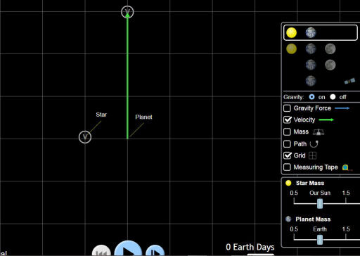
- Select "Path".
- To run the simulation, click the blue start (arrow) button. Pause the sim, when the planet has completed about 95% of its orbit.
- Use the step button (to immediate right of the start/pause button) to complete the planet's orbit. [Velocity vector should be vertical again.]
- If you need to redo the orbit, use the restart button (immediately to the left of the start/pause button).[Use scale control in upper left, if path does not fit on screen.]
- Select "Measuring Tape". Use the tape measure to measure the length of the major (horizontal axis) of the orbit.
[Might help to use tape measure upside down.] - Enter your major axis measurement in the "2A" column of your table.
- Enter the Earth Days shown in the "T" column of your table.
- Deselect "Path".
- Position the planet 2 grid spacing to the right of the star.
- Make the velocity vector perfectly vertical and 2 grid spacings long.
- Select "Path".
- Have the planet complete another orbit.
- Measure 2A. Enter its value and that of T in the table as before.
- Deselect "Path".
- Position the planet 3 grid spacing to the right of the star.
- Make the velocity vector perfectly vertical and 1 grid spacing long .
- Select "Path".
- Have the planet complete another orbit.
- Measure 2A. Enter its value and that of T in the table as before.
- Deselect "Path".
- Position the planet 4 grid spacing to the right of the star.
- Make the velocity vector perfectly vertical and 0.5 grid spacing long .
- Select "Path".
- Have the planet complete another orbit.
- Measure 2A. Enter its value and that of T in the table as before.
- Deselect "Path".
- Graph T2/A3 vs. Trial Number. [Make Trial Number the horizontal axis.]
- Is your graph a horizontal line?
- What is the difference between the largest value in the T2/A3 and the smallest?
- Calculate the % error as the difference above divided by the average value of T2/A3.
- Graph T2 vs. A3. [Make the latter the horizontal axis.]
- Is your graph a straight line? What is its slope?
- Speculate: Does T2/A3 depend on the mass of the star?
- Add a conclusion of the form: My findings support (or do not support) Kepler's Third with an error of ___%.
Lab for 09-25-25
Kinetic and Potential Energy
Objective: Confirm conservation of energy and formulas for its kinetic and potential forms.
Procedure
- Double click on the "Intro" icon above. [You may set the simulation to full-screen by clicking on the "hamburger" menu in the lower right.]
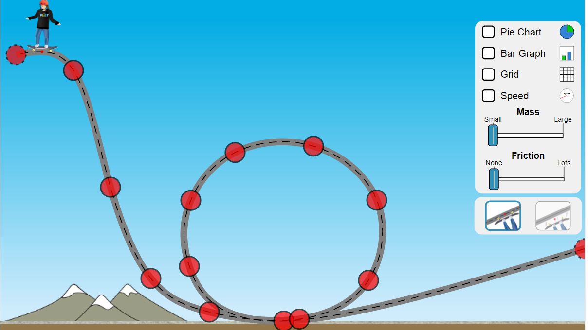
- Select "Bar Graph" and "Grid". Select "Slow Motion". Leave Mass at the position midway between small and large.
- Enter a sketch or screen capture of the parabolic track into your lab notebook.
- Position your skater near the highest position of your track. [If necessary, start the simulation my clicking the "Play/Pause" button near the bottom of the simulation.]
- Is the sum of potential energy and kinetic energy the same at all points on the track? [Pause the skater at 3 different positions. Check to see if the sum of Ep and Ek in the bar graph is the same at each position.]
- Where on the track where the potential energy is lowest?
- Where on the track where the potential energy is highest?
- Where on the track where the kinetic energy is lowest?
- Where on the track where the kinetic energy is highest?
- How is the skater's motion affected by changing his mass?
- Click on the "Friction" icon at the bottom of the simulation. Select parabolic track.
- How is the skater's motion affected by changing maximizing friction"?
- Click on the "Playground" icon at the bottom of the simulation. Set the skater's mass to "small".
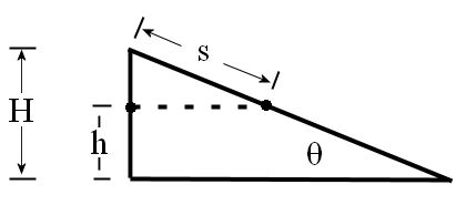
- Use the red-gray track segments to create a track that consists of two hills, as shown below.
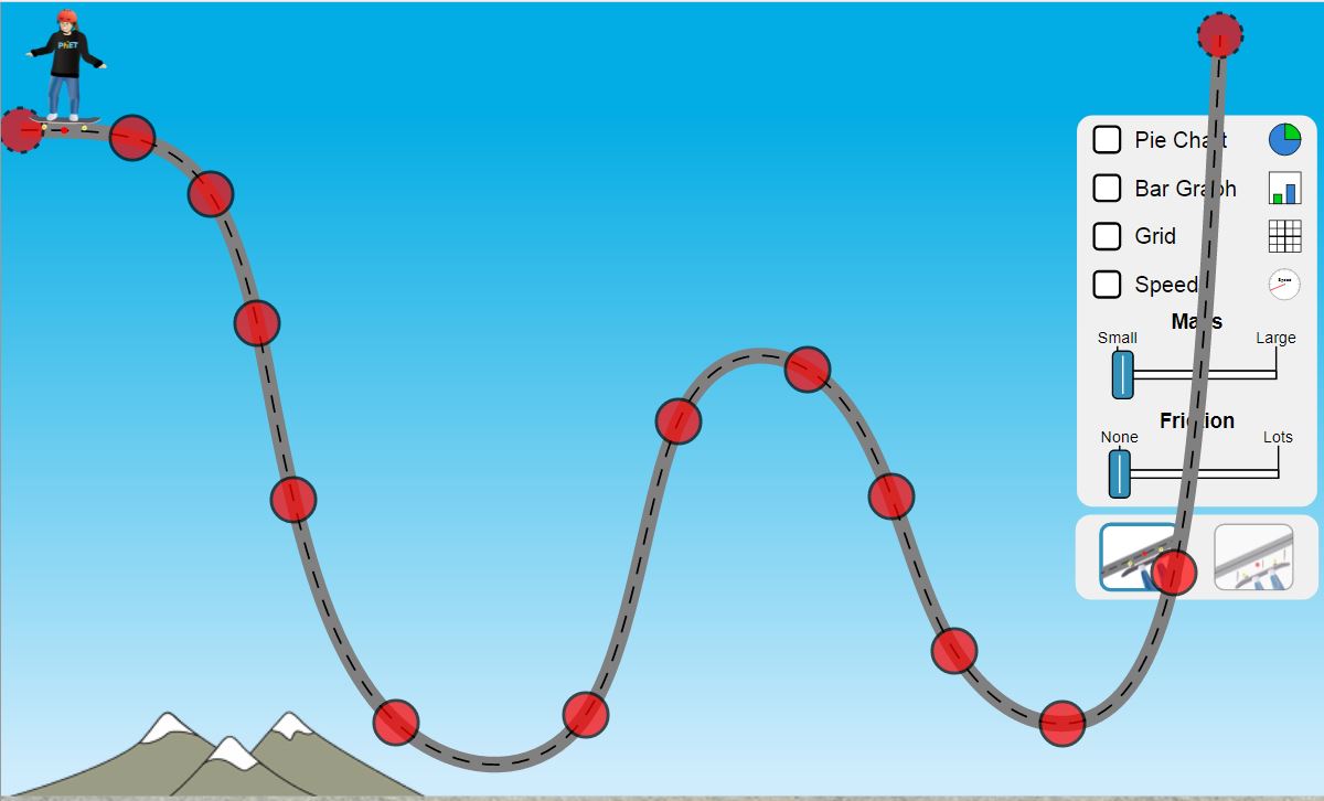
We will refer to the hill on the left as the "first hill", that on the right as the "second hill". - Click on
 to set "Roller Coaster Mode" ON.
 - Select the "Grid" to measure the heights your hills. Set Friction to "none".
- If the 1st hill has a height h1, what is the greatest height h2 of the 2nd hill that will allow the skater to traverse the 2nd hill?
- How does the total energy of the skater at the top of the 1st hill compare with its total energy at the top of the 2nd hill?
- How does the total energy of the skater at the top of the 1st hill compare with its total energy at the bottom of the 1st hill?
- Potential energy of skater: Ep = mgh. Kinetic energy of skater: Ek = mv2/2. Total energy: E = Ep + Ek. At what locations is the skater's kinetic energy greatest?
- Create a track with a loop that resembles the image below. [The loop's diameter should be about half the available space, as shown.]
- Click on
 to set "Roller Coaster Mode" OFF.
 - At what locations is the skater's potential energy greatest?
- Does the acceleration of the the skater around the loop increase or decrease if the radius of the loop is decreased?
- If the loop has a radius r and the skater has a velocity v, what is the formula that you already know that gives the acceleration of the skater around the loop?
- Let vt and vb be the speeds of the skater at the top of and bottom of the loop respectively. Set the hill to its maximum height (~8 m). What is the formula for the total energy of the skater at the bottom of the hill? [Hint: assume h = 0 at the bottom of the hill, and v = 0 at the top of the hill.]
- How does vb depend on h (the height of the hill)?
- How does the total energy at the top of the loop compare with that at the bottom of the loop? Write an equation equating the energies at the top and bottom.
- Solve the equation above for vt
- For the skater to barely remain on the track at the top of the loop, the acceleration of gravity g must equal the circular acceleration vt2/r. Solve for the loop radius rmax at which this occurs. Help
- According to your calculation, how does the diameter of the largest loop on which the skater remains on the track compare with h2?
- Use trial and error to determine how closely the simulation matches your derived expression for the maximum diameter dmax = 2rmax in terms of h?
Lab for 10-02-25
Elastic and Inelastic Collisions
Objectives:
Determine whether kinetic energy and momentum are conserved in collisions.
Test formula for final velocities of colliding objects.
Procedure:
- Click on the "Intro" icon above. Familiarize yourself with the basic operation of the simulation.
[Note reset buttons and that the menu in the lower right includes "screen shot" and "full screen".] - Create a table that looks like this:
Elastic Collisions Trial m1
(kg)m2
(kg)v1initial
(m/s)v1final
(m/s)v2initial
(m/s)v2final
(m/s)KEinitial
(J)KEfinal
(J)Pinitial
(kg-m/s)Pfinal
(kg-m/s)1 1 1 1 0 0.5 1 2 3.0 0.1 1 0 1.5 3 3 0.1 3.0 1 0 0.05 0.10 - Click "Explore 1D" icon.
- Select "More Data" checkbox to display the data panel. Place Ball 2 about 1 meter to the right of Ball 1.
- For Trial 1, enter the values shown in the table for the masses and initial velocities for Balls 1 and 2.
- Select "Kinetic Energy", "Velocity", and "Values" checkboxes.
- Set elasticity to 100%.
- Click the "Play" button. Click the "Pause" button immediately after the collision.
- Record the final values for the velocities, total kinetic energy (KE), and total momentum (P).
(Note that P is the sum of the momenta shown in the data panel). - Repeat Steps 4 - 8 for Trials 2 and 3.
- Does total kinetic energy appear to be conserved?
- Does total momentum appear to be conserved?
- To what degree are your results consistent with the following formulas?
v1final = (m1 - m2)v1initial/(m1 + m2)
v2final = (2m1)v1initial/(m1 + m2)
- What approximate form do the above formulas take when m1 = m2 (Trial 1)?
- What approximate form do the above formulas take when m1 is much greater than m2 (Trial 2)?
- What approximate form do the above formulas take when m1 is much less than m2 (Trial 3)?
- Create a table that looks like this:
Inelastic Collisions Trial m1
(kg)m2
(kg)v1initial
(m/s)v1final
(m/s)v2initial
(m/s)v2final
(m/s)KEinitial
(J)KEfinal
(J)Pinitial
(kg-m/s)Pfinal
(kg-m/s)1 1 1 1 0 0.5 1 2 3.0 0.1 1 0 1.5 3 3 0.1 3.0 1 0 0.05 0.10 - Set "Elasticity" to 50%.
- Conduct three trials as above and fill out your table.
- Does total kinetic energy appear to be conserved?
- Plot the change in Kinetic energy (y-axis) vs Trial number (x-axis).
- Do the equations in Step 12 seem to hold for inelastic collisions.
- Does total momentum appear to be conserved?
- Set "Elasticity" to 0% and cause the Balls to collide.
- What happens in such a "completely inelastic" collision?
Lab for 10-09-25
Rotational Motion
Objectives: Test the formulas for torque, moment of inertia, and angular momentum.
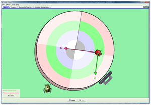
Click on the image above.
- Select the "Intro" tab.
- Figure out how to make the disk rotate. Record your findings.
- Place the insects near the center of the disk. Figure out how to speed up the disk so that they fly off. Record your finding
- Select the "Torque" tab.
- Place the lady bug near the center of the disk.
- Set the Applied Force (F) to about 1 N by moving the vertical slider (blue arrow).
- Set the Radius of Force (r) to about 3 m by moving the vertical slider (green arrow).
- Is the value of the Applied Torque (T) given by T = rF?
- Sketch the position of the Applied Force vector on the disk.
- Click on any of the "Go!" buttons.
- Does the disk seem to spin faster and faster? [Does the lady bug fly off of it?]
- Select the "Moment of Inertia" tab.
- Set the Applied Torque to about 1 N-m by moving the vertical slider (blue arrow).
- Set the inner radius to 0 m, outer radius to 4 m, mass to 0.15 kg, Force of brake to 0.
- Click on any of the "Go!" buttons.
- How does the moment of inertia (I) compare to the formula I = (MR2)/2 (where M =platform mass; R = outer radius) ?
- Convert the angular acceleration of the platform to rad/s/s by dividing it by 57.3 deg/rad
- How does the torque compare to the formula T = Iα (where α = angular acceleration in rad/s/s)?
- Select the "Angular Momentum" tab.
- Set the Angular Velocity to about 100.
- Convert the angular velocity to rad/s by dividing by 57.3 deg/rad
- Click on any of the "Go!" buttons.
- How does the angular momentum (L) compare to the formula L = Iω (where I = moment of inertia, ω = angular velocity in rad/s)?