View the line charge again:
- Setup: Charged line
- Color: field magnitude
- Floor: equipotentials
- Display: Field Vectors
- Mouse = Surface Integral
Use the mouse to create a box. [The quantity of flux passing through the box is shown in the lower left.]
- Record the flux through 3 different boxes that do not contain the central line charge.
- Record the flux through 3 different boxes that do contain the central line charge.
- Are your results consistent with Gauss' Law?
Part III: Applying the Electric Field
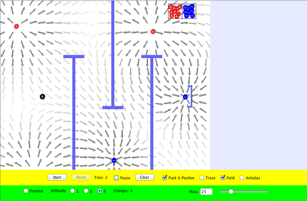
Click to Run
- Start the simulation. Note the electric charge of the puck. Your objective is to place charges (from the box in the upper right) so that the puck reaches the goal.
- Set mass to its maximum value (100).
- Select "Practice".
- Place a positive charge directly to the left of the puck.
- Click "Start". Observe that the puck enters the goal.
- Try to achieve goals for each difficulty level.
- For each difficulty level, sketch or screen capture the arrangement of charges that worked for you.
- To get you started, here is an arrangement that works at Difficulty Level 2

Part IV: OPTIONAL Gel Electrophoresis
Please go to this link and do the following lab:
- Gel Electrophoresis
- Please summarize the basic steps required to carry out gel electrophoresis. [Please number your steps.]
- What would happen if the electric field were very much stronger?
Lab for 1-22-26
The Parallel-Plate Capacitor
Objective: To compare the measured properties of a parallel plate capacitor to those predicted by theory
- Click on the "Capacitance" icon above to start the simulation.
- Check all 7 of the checkboxes in the two panels.
- Set the battery to 1.5 Volts by moving the switch as high at it goes.
- Position the voltmeter's red probe so that it contacts the wire connected to the top of the battery. Position the voltmeter's black probe so that it contacts the wire connected to the bottom of the battery. What does the voltmeter read? How does this compare to the voltage of the battery?
- Slide the switch on the battery. Observer the corresponding voltage on the volt meter.
- Create a table that looks like this:
EXPERIMENT
Battery Potential
(Volts)
Plate Separation
(mm)
Plate Area
(mm2)
Capacitance
(Farads)
Plate Charge
(Coulombs)
Stored Energy
(Joules)
Electric Field
(Volts/meter)
0.20
10
100
0.50
10
100
1.0
10
100
1.5
10
100
1.5
7.5
100
1.5
5.0
100
1.5
5.0
200
1.5
5.0
400
- Use the sliding switch on the battery and the two double-sided arrows to set the battery potential, plate separation, and plate area
to the values shown in the first row of the table above.
- Read the values shown for the capacitance, top plate charge, and stored energy to fill out the corresponding
entries in the first row of the table above.
- Calcuate the electic field between the plates by using the formula
E = V/d
where V = voltmeter's reading (in Volts)
d = the plate separation converted to meters.
Enter this value into the right-most column of the first row.
- Repeat the last 3 steps for the remaining rows of the table above.
- Create table that looks like this:
THEORY
Battery Potential
(Volts)
Plate Separation
(mm)
Plate Area
(mm2)
Capacitance
(Farads)
Plate Charge
(Coulombs)
Stored Energy
(Joules)
Electric Field
(Volts/meter)
0.20
10
100
0.50
10
100
1.0
10
100
1.5
10
100
1.5
7.5
100
1.5
5.0
100
1.5
5.0
200
1.5
5.0
400
Fill out the Theory table using the following formulas.
C = A/(4πkd) (That wierd symbol after the 4 is pi)
Q = CV
U = (1/2)CV2
E = V/d
V = Battery Potential
d = Plate Separation
A = Plate Area
C = Capacitance
Q = Plate Charge
U = Stored Energy
E = Electric Field
k = 8.99 x 10⁹ N m2/C2
Remember to convert mm to meters
Lab for 1-29-26
Voltage, Current, and Resistance
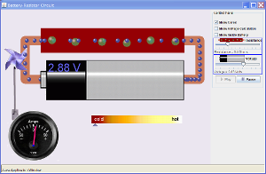
Click to Run
- Set the battery voltage to about 10 Volts (record your exact voltage).
- Create a table like this one
Row R I IR IV Hotness (%)
1 2 3 4 5
- For each row in the table above,
- choose a value of R
- read I (from the ammeter)
- calculate IR
- calculate IV
- estimate hotness (from 0 to 100%)
- Plot I vs R (R on horizontal axis)
- Describe the depedence of I on R. Guess the formula for I = I(R).
- Plot IR vs row number (row number on horizontal axis)
- Is IR about constant?
- Plot IV vs Hotness (hotness on horizontal axis)
- Describe the relationship between IV and hotness.
- Create a table like this one
Row V R I IR 1 2 3 4 5
For each row in the table
- Set the battery voltage to a new value of V. Record it in the V column.
- Set the resistor's resistance to a new value R. Record it in the R column.
- Read the current I from the ammeter. Record it in the I column.
- Calculate IR. Record IR in the IR column.
- Plot IR vs V (V on the horizontal axis).
- How does IR depend on V? Guess a formula for V = V(I,R)
Use this Circuit Construction Simulation to carry out the instructions below.
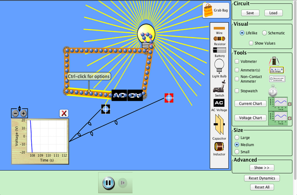
- Create a circuit that looks like this (leave the switch open).
 Hint:
Hint: 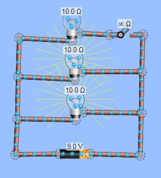
- Right click on each bulb and select show value. Record this resistance value for each bulb.
- Lower the resistance of value of one of the bulbs by half or to about 3 Ohms (whichever is smallest). Does the bulb shine more or less brightly?
- Lower the resistence of value of one of the bulbs to zero. Describe what happens.
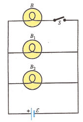
- Set the resistence of all 3 bulbs to 10 Ohms. Guess whether the brightness of the lower bulbs will change when the switch is closed.
- Test your prediction. Explain the result. [Hint: Brightness = IV = (V/R)V =V2/R. Did V or R change for the lower bulbs, when the switch was closed? ]
- What happens to the brightness of a bulb, when a resistor is placed next to it in the circuit?
- Use the ammeter and volt meters to explain why? [Hint: Brightness = IVB, where VB is the voltage difference between terminals of the bulb, and I is current through the bulb.]
- What is the value of the resistor? [Hint: Create a little circuit with just wire, the battery, and a resistor. Use Ohm's Law (V=IR), the ammeter and the voltmeter. OR go here.]
Lab for 2-05-26
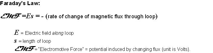
Faraday's Law
Objective: Understand Faraday's Law
.
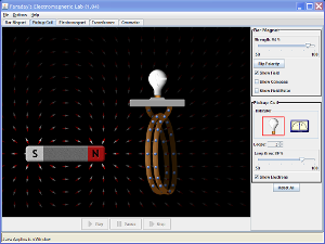
- In the simulation above, place the bar magnet well to the right of the coil so that the north pole of the magnet is closest to the coil. Select the single coil arrangement. Check the "Field lines" box. Note the number of magnetic field lines entering the coil.
- Very slowly move the magnet leftward so that it enters the coil. Has the number of magnetic field lines entering the coil increased? Does this mean that the magnetic flux through the loops that constitute the coil has increased?
- Slowy return the magnet to its original position. Now rapidly move it leftward into the coil. Did the voltmeter register a spike in voltage? Does the spike in voltage persist after the magnet comes to rest within the coil? Is this observation consistent with Faraday's Law? What was the sign of the spike?
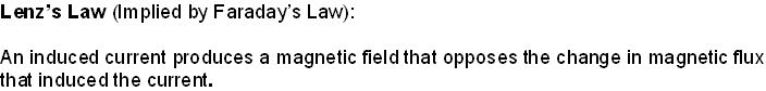
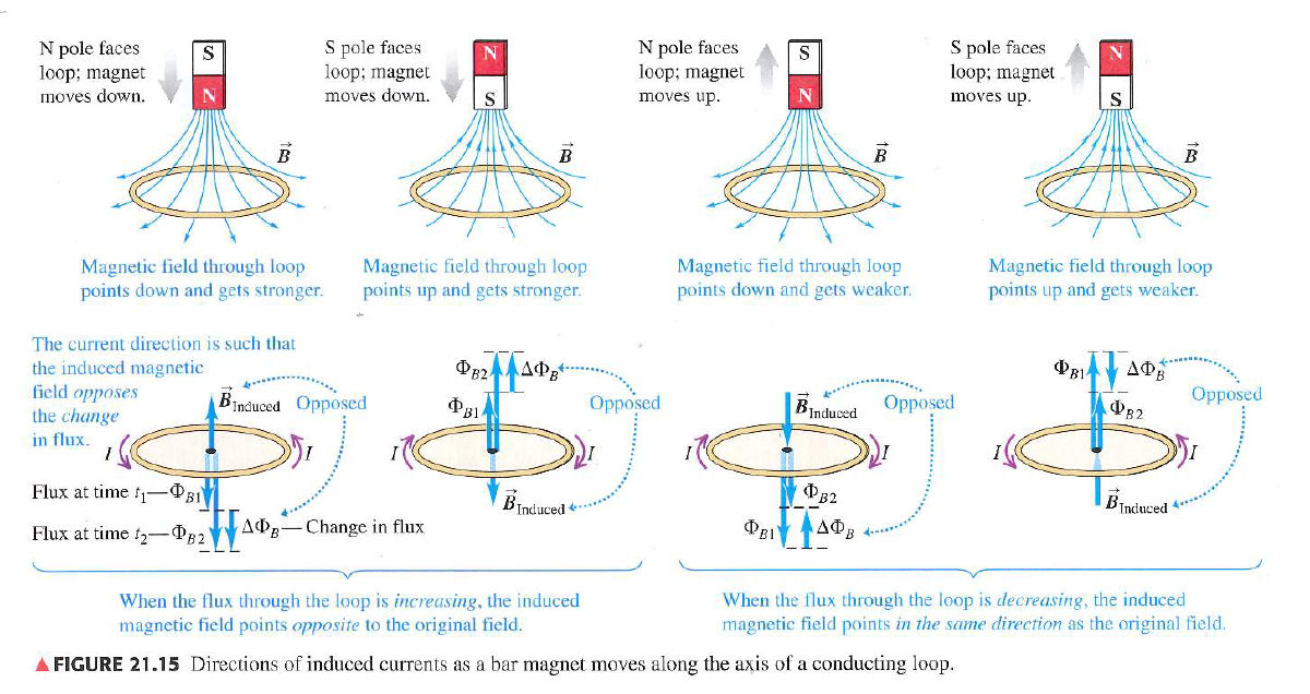
- In what direction must the magnetic field induced (by the rapid insertion of the bar magnet) point in order to oppose the resulting change in the magnetic flux? [Consult the figure below that illustrates Lenz's Law].
- Insert the bar magnet within the coil (orient the magnet's north pole to the left of its south pole). Rapidly yank the magnet to the right. Did you observer a voltage spike. What was the sign of the voltage spike. Is this consistent with Lenz's Law?
- Select the two-coil arrangement. Which creates the greater voltage, passing the magnet through the 4-loop coil or the 2-loop coil? Why?
- Click on the icon below to start the Faraday's Electromagnetic Lab simulation.
Click to Run
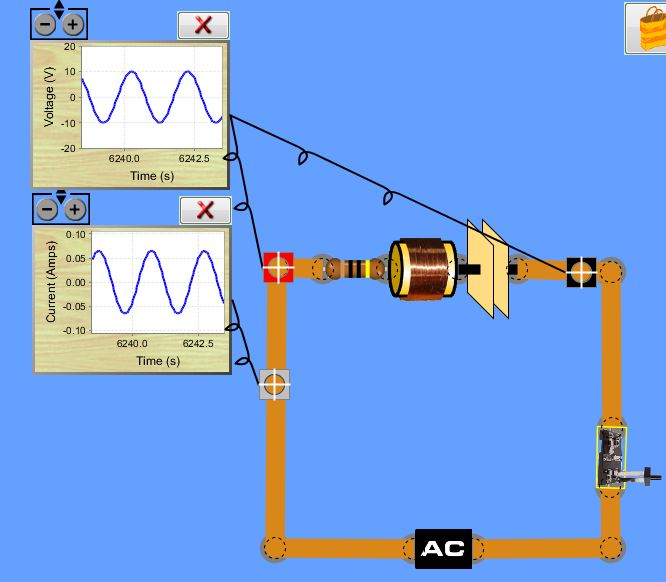
- Select the "Transformer" tab. Set the Current Source to "DC". Check "Show Field" and "Show Electrons". Set loop area to 100%. Set the Pickup Coil Indicator to Voltmeter (instead of light bulb). Is the magentic flux passing through larger loop changing? What is this there a voltage being induced in the larger loop?
- Use the slider on the battery to rapidly switch its polarity. Does cause the magnetic flux through the larger loop to change? Does this result in a voltage spike?
- Set the Current Source to "AC". Experiment with the sliders on the AC Current Supply that increase peak current and current frequency (the inverse of the period of the sine wave shown). Does the magnitude of the voltage spikes increase as the AC Current Supply's peak current (vertical slider) is increased. Does the magnitude of the voltage spikes increase as the AC Current Supply's frequency is increased? Does this seem to follow from Faraday's Law?
- Does the changing current in the first loop (powered by the AC Current Supply) seem to inducea voltage in the second (larger) loop? Is the current associated with this induced voltage AC or DC (the the direction of the current in the large loop seem to alternate)? What is the name for the phenomenon in which a changing current in one loop induces a voltage in another loop? [Remeber the last lecture.]
- Set the Pickup Coil indicator to "light bulb". Move the smaller coil into the larger one. Does the light bulb glow more brightly?
- Use the slider to set the loop area of the larger coil to 20%. Does the light bulb glow more brightly? Why? [Hint: Consider the magentic field within the smaller loop and outside of the smaller loop. These point in opposite directions (so their effects partially cancel). When the larger loops is reduced to the size of the smaller loop, the magnetic field exterior to the smaller loop is also exterior to the larger loop. So there is no longer a partial cancellation occuring within the larger loop.]
- Set the simulation tab to "Generator". Set the Pickup Coil Indicator to the voltmeter. Does
the voltage produced increase as the rotation rate of the paddle wheel is produced?
- Is the voltage produced by this generator AC or DC?
- How does the voltage produced change as the the area of the loop is decreased? Explain this.
[Hint: (Rate of change of flux) = ((Max Flux) - (Min Flux))/(rotation period). (Max Flux) = BA. (Min Flux) = -BA.]
- Summarize your conlusions as usual.
Lab for 2-19-26
DC Circuits
Objective: Investigate the properties of RC, LR, LC, and LRC circuits
Note: Such circuits are used to model the electrical properties of various biological structures such as neurons and cell membranes.
Click to Run
This is free form lab.
Developing your own procedure is an important skill that you will need to perform well in a real-world laboratory.
In this, lab your assignment is to use a circuit simulator explore the properies of 4 circuits.
To get you familiar with the simulator, you are provided explicit instructions for setting up the LC circuit.
For the LR, RC, and LRC circuit, step-by-step instructions are not provided. For these circuits you only need to
- Draw (or screen capture) the circuit that you have created.
- Draw the resulting current (I) vs. time (t) curve (put time on the horizontal axis).
- Ensure that you note the values of R, L, or C associated with your I vs. t graph.
- Describe the change in your graph that results from changing R,L, or C.
- Be sure to measure and compare to theory the
- charge/discharge time for RC circuit
- time to steady current for LR circuit
- period (or frequency) for LC circuit
Part I: LC Circuit
- Start the simulator.
Click on icon above. Double click square labeled "RLC" that appears. Figure out how to drag circuit elements into place.
- Create LC circuit that looks like this.
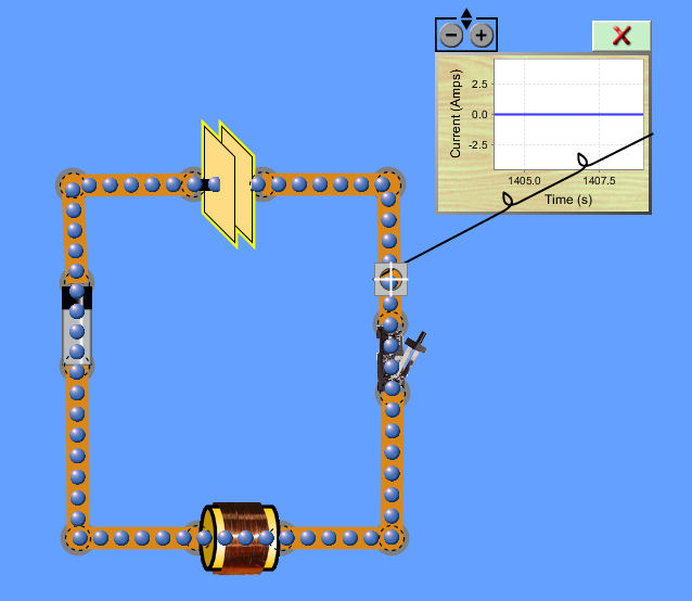
- Ensure that the switch is open. [Slide switch handle outward with mouse.]
- Change the battery's potential to 50 Volts. [Right click on battery; select "Change Voltage".]
- Set inductance to 35 Henries. [Right click on inductor; select "Change Inductance".]
- Set capacitance to 0.09 Farads. [Right click on capacitor; select "Change Capacitance"]
- Close the switch.
- Allow the capacitor to become fully charged. (should only take a few seconds).
- Open the switch.
- Remove the battery. [Right click on battery; select "Remove"]
- Eliminate the gap in the circuit. [Join the ends of the wires, which were previously connect to the ends of the battery, to each other.]
- Close the switch.
- Observe the behavior of the circuit. [Use the (-) and (+) buttons on the Current vs. Time grapher to keep the maximum current applitude near the top of the grapher's window.]
- Does current oscillate? If so, at what what is the period of the oscillation.
- What is the maximum current.
- What happens if you make L and C as small as possible?
- Fill out the following table for 4 choices for an L,C pair.
L (Henries)
C (Farads)
Period (Seconds)
Frequency (Hz)
=1/Period
- Is your data consistent with the frequency formula
f = 1/(2π√ LC )
Part II: LR Circuit
Part III: LC Circuit
Part IV: LRC Circuit
Lab for 2-26-26
AC Circuits
Objective: Verify the formulas for reactance, impedance, and phase lag in AC circuits
Procedure
Click to Run
- Start the circuit simulator by clicking on the link above. After a new screen appears, click on the square labeled "RLC".
- Use the simulator to contruct a circuit shown below. Be sure to attach the voltage and current meters as indicated
(so that red volt meter's probe is on same side of the circuit element as the current meter's probe).
Leave the switch open as shown.
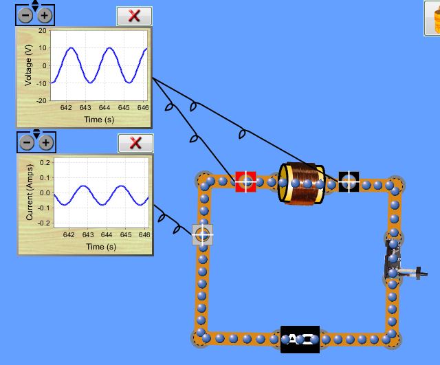
- Right click on the AC power source to set the frequency to 0.5 Hz and the peak AC voltage to 10 V.
- Right click on the inductor to set its inductance to 50 Henries.
- Calculate the reactance X of the inductor.
	X = 2πfL  	(=  159.5 Ohms)

	where f = 0.5 Hz
	      L = 50 Henries
- Calculate the expected peak current I.
	I = V/X		(= 10/159.5 = 0.0627 Amps)

	where V = 10 Volts
- Use the "+" or "-" buttons on the voltage meter to ensure that the meter's voltage scale includes
the peak voltage to which the AC power supply is set.
- Use the "+" or "-" buttons on the the current meter to ensure that the meter's current scale includes
the peak current calculate in step 6.
- Create the table below. Enter the following value into the first row
	Frequency:  		0.5
	Reactance		159.5
	Voltage			10
	Current (Theory)	0.627
Circuit Element
Frequency
(Hz)
Reactance
(Ohms)
Peak Voltage
(Volts)
Peak Current
(theory)
(Amps)
Peak Current
(observed)
(Amps)
Phase Shift
(theory)
(degrees)
Phase Shift
(observed)
(degrees)
inductor
(50 Henries)
0.5
10
+90
(lead)
capacitor
(0.1 Farad)
0.5
10
-90
(lag)
resistor
(10 Ohms)
0.5
10
0
(in phase)
- Close to switch in your circuit. Wait a few seconds to allow complete sinusoidal wave forms to appear on both the current and
voltage meters.
- Pause the simulation using the button at the bottom of the screen.
- Obtain the peak current as follows.
       * On the current meter, read the current reach by the waveform when it is at its maximum value.
       * Read the current reached when the waveform is at its minimum value.
       * The peak is half the difference between these two values.
         (e.g. Imax = 0.6,  Imin = -0.8, Ipeak = (0.6 - (-0.8))/2 = 0.7).
       * Enter this value under "Current Expected" for the circuit element.
- Obtain the phase shift as follows.
	* On the current meter, estimate the time value Tc associated with a minimum of the waveform that is
          located near the center of the meter's display window  (eg  Tc = 345.8).
	* On the voltage meter, estimate the minimum Tv of the waveform that is closest in time to Tc (e.g. Tv = 345.2).
	* Calculate the phase shift Φ in degrees:

			Φ = (Tc - Tv)×f×360   	e.g. (345.8 - 345.2)×0.5×360 = 108 degrees
	     		If Φ > 0 → phase lead
			If Φ < 0 → phase lag
			If Φ = 0 → in phase


	* Enter the phase shift in the "Phase Shift Observed" column for the circuit element (e.g. 108 deg lead)
- Replace the inductor in your circuit with a capacitor, and repeat steps 1 - 13 with the following exceptions.
	* Use the reactance formula for a capacitor:  X = 1/(2πfC)
	* Use the same table and enter data in the "capacitor" row.
- Replace the capacitor in your circuit with a resistor, and repeat steps 1 - 13 with the following exceptions.
	* Use the reactance formula for a capacitor:  X = R
	* Use the same table, but enter data in the "resistor" row.
- Calculate the average error percentage for your phase shifts = 100(Φobserved - Φtheory)/Φtheory
- Calcuate the average error percentage for your currents = 100(Iobserved - Itheory)/Itheory
- Identify source of error.
- Construct the series R-L-C circuit shown below.
- Calculate the impedance Z of the circuit
	Z = sqrt( (XL - XC)2 + R2 )

	where  XL = 2πfL
	       XC = 1/(2πfC)
- Calculate the expected peak current.
Ipeak = V/Z.
- Obtain the observed value of Ipeak.
          Run the simulation.
	  Obtain Ipeak (See step 12).
	  How does this compare to the theoretical value for Ipeak (step 21).
Lab for 03-05-26
Reflection and Refraction
Objective: Determine the implications of Snell's Law
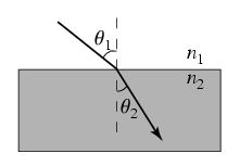
- Please click on "Intro" in the square labeled "Bending Light" above . Set the Laser View to "Ray". Set the Material above and below the interface to "Custom".
- Use the sliders to find by trial and error the the relationship between n1 (index of refraction for upper material) and n2 (index of refraction for lower material) that ensures that the angle of incidence θ1 equals the angle of refraction θ2.
- Should the simulation show a reflected beam in this case? [Hint: There would be no interface in this case.]
- Set n1=1.5 and n2=1.0. Find the smallest angle of incidence (the "critical angle") at which no refraction -- i.e. "total internal reflection" -- occurs
- Use Snell's Law to derive an expression in for the angle at which this will occur for any choice of n1 and n2.
- Choose 4 pairs of n1 and n2 with n1 > n2. Use the simulator to find the critical angle for each pair.
- How do your values for the critical angle compare to your formula?
- Switch the Laser View to "Wave". Set n1=1.0 and n2=1.6. Are the wavelengths of incident and refracted waves the same?
- Are the frequencies of the incident and refracted waves the same? [Count the number of line that go past a fixed point in 10 seconds.]
- Are the speeds of the incident and refracted waves the same?
- Use the "Speed Tool" (under the "More Tools" tab) to obtain the speed v1 of the incident wave and the speed v2 of the refracted wave.
- How does the ratio of these speeds, v1/v2, compare to n2/n1?
Lab for 3-12-26
Optics & Interference
Objective: Confirm the Thin Lens Equation and the Double Slit Interference Equation
PART A: Optics
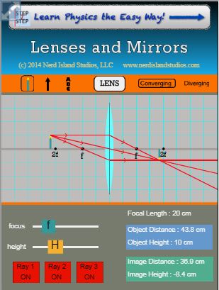
Click on the image to the left to reach the page containing the geometric optics simulator.
Once there, you may resize the simulator to fullscreen (by clicking on its upper left corner).
This is a free form lab. Your objective is to use the simulation above to confirm the the the Thin Lens Equation and the Magnification Equation that follows from it.
FOR LENSES
Lens equation: 1/p + 1/q = 1/f
p = distance from lens surface to object (p > 0 always) q = distance from lens surface to image f = distance from lens surface to focal point if lens type is DIVERGING (Concave), f < 0 if lens type is CONVERGING (Convex), f > 0 if q is behind lens , q > 0 and image is REAL if q is in front of lens, q < 0 and image is VIRTUAL Magnification = (image height)/(object height) = -q/p if magnification > 0, image is not inverted if magnification < 0, image is inverted if |magnification| > 1, lens magnifies the object if |magnification| < 1, lens shrinks the object
Please be sure to create a table that looks something like this:
f (cm)
p (cm)
himage
hobject
qexp
qtheory
=(1/f - 1/p)-1
Mexp
=himage/hobject
Mtheory
=-q/p
Errorq
=100x(qtheory - qexp)/qexp
ErrorM
=100x(Mtheory - Mexp)/Mexp
You would proceed as follows.
- Choose an focal length f and an object distance p.
- Measure the image distance q.
- Measure the image height himage and the object height hobject.
- Calculate the experimental magnification M (take the ratio image-to-object heights)
- Complete the table row by entering theoretical values for q and M and calculation the error.
- Repeat for another value of p. [You may keep f constant.]
PART B: Interference
Select the "Interference" icon above.
Your objective here is to verify the double slit formula for the location of dark fringes (locations of destructive interference on the right edge of the simulation).
Only measure the location of the first dark fringe on either side of the central bright region (of constructive interference).
Formula for location of first dark fringe:
y = L(1/2)λ/d
y = distance above center of central bright spot (measured at the right edge)
L = distance between the point of wave creation and the right edge.
λ = wave length
d = separation between wave sources.
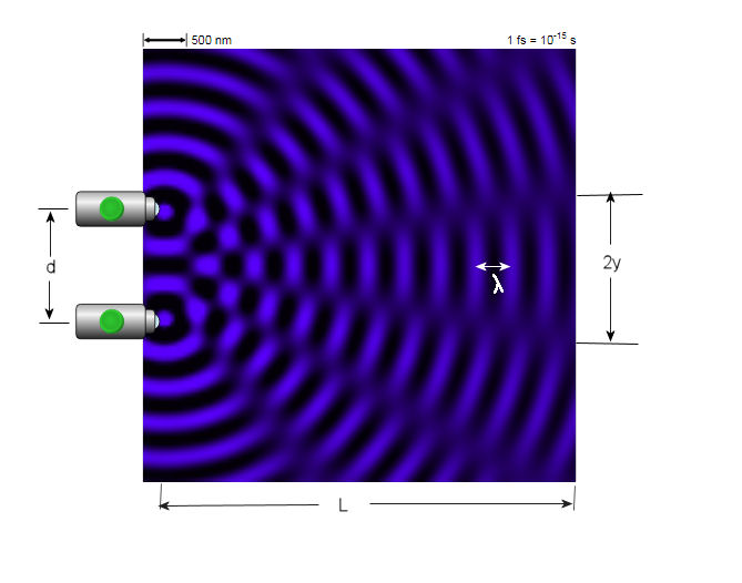
Measure y as shown above. Compare the value you measure with that resulting from the formula.
You may choose whichever medium (water, sound, or light) you prefer.
Advice: It might be easier to use high frequencies and high amplitudes.
Lab for 3-19-26
Time Dilation
Objective: Understand why motion-induced time dilation.
Definitions
light clock -- clock consisting a pulse of light that "bounces" back and forth endless between two mirrors.
time dilation -- the lengthening, perceived by a stationary observer, of the time between ticks of a clock in motion.
Procedure
- Use the simulator above or go here.
- Measure the speed of light using Jack's stationary clock.
Select trace
Click the green start button.
Click pause when Jack's light pulse reaches the top mirror.
Measure the length Lk of the white trace of the Jack's pulse's path. Use a physical ruler applied to your computer screen. [Result will be in inches or cm.]
Lk = ___________________
Record the time elapsed according to Jack's (stationary clock) upper right.
Tk = __________________
Calculate speed of light c for this simulation [Units: cm/sec or in/sec]
c = Lk/Tk
- Set the MOVING CLOCK VELOCITY slider to 0.5c.
[This sets Jill's speed relative to Bob. c = speed of light]
[Tip: Click on the slider and use you keyboard's left and right arrow buttons to enter a precise value.]
Jill's speed = ____________ = v
- Ensure that "Trace" is selected, by clicking the TRACE button if it is unchecked.
- Click the green START button.
- Click the PAUSE button the moment that Jill's light pulse touches the upper mirror (its turn-around point).
[Practice a couple of times.]
- Record the time elapsed according to Jack's clock and that according to Jill's (upper right corner).
Jack's clock reads: ___________ = Tk, Jill's clock reads: ______________ = Tl
- Use a ruler to measure the length the white pulse trace between Jill's starting point and it's upper-most point (where pulse touches mirror).
length of Jill's half-tick pulse path: _________________ = Ll
- Calculate the speed of the pulse in Jill's clock (in Jack's reference frame).
Ll/Tk: _______________ = speed of light in Jill's clock
- Repeat Steps 3 - 10 for at least 3 additional choices for Jill's speed (such as those suggested below), and complete the table.
Theoretical Time Dilation Formula:
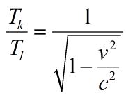
where v = Jill's speed.
[Example: Let v = 0.5c. Then Tk/Tl = 1/sqrt(1 - 0.52) = 1.15]
Jill's Speed
Jill's pulse
trace length (in or cm)
Jill's clock
reading (s)
Jack's clock
reading (s)
Simulation's c
(in/s or cm/s)
Time Dilation
Measured
Time Dilation
Theoretical
v
Ll
Tl
Tk
Ll/Tk
Tk/Tl
Tk/Tl
0.50c
0.70c
0.90c
0.95c
- Graph the experimental value of Tk/Tl vs Jill's speed (in units of c).
- Overlay the theoretical plot of Tk/Tl vs Jill's speed on the same graph.
- Do the experimental and theoretical graphs seem to agree?
- Does Tl increase relative to Tk as Jill's speed increases?
- Would "Time dilation" seem to be an apt term for the motion-induced increase in the duration of clock tick's?
- Graph the speed of light verses Jill's speed by using your measured ratios of the length of light's path to Jill's mirror to the time elapsed
according to Jack's clock. Graph 5 data points. Let the first be the speed of light when Jill is stationary (0.00c), which is the same
as what you calculated for the stationary Jack in Step 2 above. For the other 4 data points, use the 4 values in the Ll/Tk column of the
table above. Put Jill's speed be on the horizontal axis and Ll/Tk, your speed of light measurement, on the vertical axis.
- Does the speed of light measured using Jill's clock match that in Jack's? Does the speed of light seem to be constant?
- If a (half) tick of Jill's moving clock takes longer than a (half) tick of Jack's stationary clock, how is it that
the speed of light has the same value when measured using either light clock?
- Discuss sources and magnitude of error.
- Write a conclusion:
The theoretical formula for time dilation does not appear to be correct.
OR
The theoretical formula for time dilation appears to correct to within _______%.
Lab for 3-26-26
The Photoelectric Effect
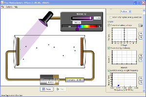
Click to Run
Objective: Calculate Planck's constant and the "work functions" of a few metals.
Background Facts:
- Shining light on a metal surface can cause electrons to be ejected from the metal.
- For a particular metal, there is a maximum wavelength of light beyond which no electrons are ejected.
- When the wavelength of light exceeds this maximum (for a particular metal), electrons fail to be ejected even if the intensity of light is arbitrarily increased.
- The last sentence is inconsistent with classical physics.
Derivation of Main Formula
total energy = (kinetic energy) + (potential energy)
total energy = hf (h = Planck's constant = 4.14 x 10⁻¹⁵eV; f = frequency of incident light)
kinetic energy = mv2/2 (m = electron mass; v = electron velocity)
potential energy due to work function = φ
potential energy due to electric field = e(V/d)x (e = charge on electron = 1.60 x 10⁻¹⁹ C; d = separation between plates; x = distance of electron from left plate; V = applied voltage)
So,
hf = mv2/2 + e(V/d)x + φ
If voltage is set so that electrons stop (v=0) just before reaching the right plate (x=d), we have
hf = eV + φ
Or,
V= (h/e)f - φ/e where f= c/λ
Procedure
- Set the battery voltage to zero and the target to sodium. Set the wavelength so that no electrons are ejected. Increase the intensity of light to 100%. Does this cause electrons to be ejected?
- With the battery voltage set to zero and the target set to sodium, find the longest wavelength λ at which electrons are emitted.
- Calculate the work function using φ = hc/λ (i.e. value φ from above equation with V = 0)
- Repeat for copper and zinc.
- Compare your results with this table.
- For sodium, choose a low wavelength for which electrons are emitted. Find the voltage at which electrons just miss making it to the electrode on the right.
- Repeat last step for 2 more wavelengths. Calculate the frequencies corresponding to these wavelengths.
- Plot the 3 (frequency, voltage) pairs and graph a line through them (V on the vertical axis, f on the horizontal).
- Use the main formula derived above to obtain a value for Planck's constant and the work function.[help]
- Compare your results with the known values of Planck's constant and sodium work function.
Lab for 4-02-26
Nuclear Fission
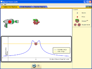
Click to Run
Purpose: To the determine the degree to which Uranium must be enriched in order to become fissionable. Definitions:
fissionable isotope An isotope that undergoes nuclear fission, i.e. one that splits when an energetic neutron collides with it. fissionable sample A fissionable sample of uranium is one that will undergo a chain reaction when it is exposed to neutrons. enrichment the increasing of the fraction of fissionable isotopes in a sample of nuclei (e.g., increasing the fraction of U-235 isotopes in a sample of Uranium nuclei.)
 U-235	is a fissionable isotope
 U-238  is not a fissionable isotope.
 U-239  is not a fissionable isotope.

It is possible to prepare a sample that contains only U-235 an U-238 nuclei.
We can define the impurity of the sample (i.e. the fraction of its nuclei that are not fissionable), follows
Impurity = (N238/(N235 + N238)) x 100
where
 N235 = the number of U-235 nuclei in our sample.
 N238 = the number of U-238 nuclei in our sample.


 Your objective is to determine largest impurity that will permit a chain reaction to occur.

Procedure

1. Create a table that looks like this.
N238
N235
Impurity (%)
U-235 Nuclei Fissioned (%)
0 100 5 100 11 100 25 100 39 91 52 78 65 65 71 59 78 52 84 46 91 39 100 25 100 11
2. Start the simulation.  Go the "Chain Reaction" tab.  For each row of your table, proceed as follows:

3. Set the number of U-235 nuclei to that in the first column.
     [Tip: Click on the slider, then use the left and right arrow keys of your keyboard for greater precision.]

4. Set the number of U-235 nuclei to that in the second column.

5. Calculate the Impurity and enter it in the third column.

6. Fire the "neutron gun" 3 times in rapid succession.

7. Record "235U nuclei fissioned" displayed by the simulation (lower right) in the fourth column.

8. Click the "Reset Nuclei" button, if it is visible.

9. Repeat Steps 3 to 8 for the remaining rows of your table.

10.  Plot "Percentage U-235 Fissioned" vs. "Impurity of Sample".  [Let the horizonal access be "Impurity"].

11.  If you'd like to investigate additional impurity levels, use the blank rows to your table.
        [Note: The simulation restricts N235 and N238 as follows: 1) they must both be less
        that 100, and their sum must be less than 130.]

12. What is the highest level of impurity that will reliably permit a chain reaction to occur?

13. Reseach: What device is commonly used to enrich uranium (i.e. to increase its purity)?
       [Hint: It involves spinning, and it's name begins with "c".]
Lab for 4-09-26
Radioactive Dating
Click to Run
Objective: Demonstrate the principle of radioactive dating.
Background Information:
Radioactive decay formula: N = N02-t/τ
We can solve for t to obtain: t = -τlog(N/No)/log(2)
No = initial number of undecayed nuclei
N = number undecayed nuclei at time t
τ = half life of nuclei
[Note: log(2) = 0.301]
Procedure:
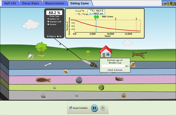
- Download the simulation by clicking on the image above. Start the simulation. Select the "Dating Game" tab.
- Create the following table:
Object
Probe Type
Probe Reading
Object Age from Simulation
Object Age from Formula
- Select Carbon-14 as the probe type.
- Move the probe (which looks like a microphone) onto the house so that a green popup box appears.
- In the yellow graph, slide the vertical line horizontally until the 14C percentage matches, as closely as possible, the probe's reading (shown in the black box attached to the probe wire).
- Read the estimated age of the house from the small light yellow box within the yellow box containing the graph.
- Enter this value into the "Estimate age of House" text box in the green popup box.
- If the simulation did not reward you with a green happy face, repeat the steps aboveIf the simulation did not reward you with a green happy face, repeat the steps above.
- Enter the following into the first line of your table:
Object
Probe Type
Probe Reading
Object Age from Simulation
Object Age from Formula
House
Carbon-14
99.1%
77 yrs
- Use the formula above to calculate the age of house:
t = -(5730)log(0.991)/0.301 = 74.7
Enter this value in the "Object Age from Formula" column of your table.
[Note: 5730 is the half life of Carbon-14.]
- Complete your table by repeating the above for at least one object from each of the subterranean geological layers shown.
[Note: You will need change your probe type to obtain the ages of the deeper objects.
Be sure to use the correct half life in the formula.]
- How closely did the simulation match the formula, withing 10%, 5%, 1%, or other?
- Use this list to find the radioactive isotopes with half lives closest to
- 105 years
- 106 years
- 107 years
- 108 years
- Why can't you use Carbon-14 dating to determine the age of object that is over 100 million years old?
| Click to Run |
- Click on the "Capacitance" icon above to start the simulation.
- Check all 7 of the checkboxes in the two panels.
- Set the battery to 1.5 Volts by moving the switch as high at it goes.
- Position the voltmeter's red probe so that it contacts the wire connected to the top of the battery. Position the voltmeter's black probe so that it contacts the wire connected to the bottom of the battery. What does the voltmeter read? How does this compare to the voltage of the battery?
- Slide the switch on the battery. Observer the corresponding voltage on the volt meter.
- Create a table that looks like this:
EXPERIMENT
Battery Potential
(Volts)Plate Separation
(mm)Plate Area
(mm2)Capacitance
(Farads)Plate Charge
(Coulombs)Stored Energy
(Joules)Electric Field
(Volts/meter)0.20 10 100 0.50 10 100 1.0 10 100 1.5 10 100 1.5 7.5 100 1.5 5.0 100 1.5 5.0 200 1.5 5.0 400 - Use the sliding switch on the battery and the two double-sided arrows to set the battery potential, plate separation, and plate area to the values shown in the first row of the table above.
- Read the values shown for the capacitance, top plate charge, and stored energy to fill out the corresponding entries in the first row of the table above.
- Calcuate the electic field between the plates by using the formula
E = V/d
where V = voltmeter's reading (in Volts)
d = the plate separation converted to meters.
Enter this value into the right-most column of the first row. - Repeat the last 3 steps for the remaining rows of the table above.
- Create table that looks like this:
THEORY
Battery Potential
(Volts)Plate Separation
(mm)Plate Area
(mm2)Capacitance
(Farads)Plate Charge
(Coulombs)Stored Energy
(Joules)Electric Field
(Volts/meter)0.20 10 100 0.50 10 100 1.0 10 100 1.5 10 100 1.5 7.5 100 1.5 5.0 100 1.5 5.0 200 1.5 5.0 400
Fill out the Theory table using the following formulas.
C = A/(4πkd) (That wierd symbol after the 4 is pi)
Q = CV
U = (1/2)CV2
E = V/d
V = Battery Potential
d = Plate Separation
A = Plate Area
C = Capacitance
Q = Plate Charge
U = Stored Energy
E = Electric Field
k = 8.99 x 10⁹ N m2/C2
Remember to convert mm to meters
- Set the battery voltage to about 10 Volts (record your exact voltage).
- Create a table like this one
Row R I IR IV Hotness (%) 1 2 3 4 5 - For each row in the table above,
- choose a value of R
- read I (from the ammeter)
- calculate IR
- calculate IV
- estimate hotness (from 0 to 100%)
- Plot I vs R (R on horizontal axis)
- Describe the depedence of I on R. Guess the formula for I = I(R).
- Plot IR vs row number (row number on horizontal axis)
- Is IR about constant?
- Plot IV vs Hotness (hotness on horizontal axis)
- Describe the relationship between IV and hotness.
- Create a table like this one
For each row in the tableRow V R I IR 1 2 3 4 5 - Set the battery voltage to a new value of V. Record it in the V column.
- Set the resistor's resistance to a new value R. Record it in the R column.
- Read the current I from the ammeter. Record it in the I column.
- Calculate IR. Record IR in the IR column.
- Plot IR vs V (V on the horizontal axis).
- How does IR depend on V? Guess a formula for V = V(I,R)
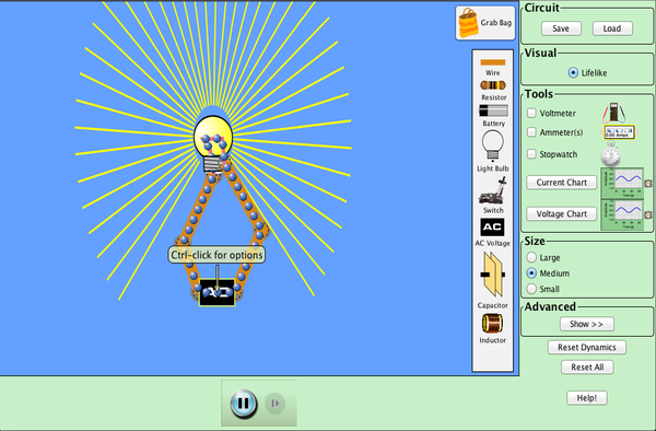
- Create a circuit that looks like this (leave the switch open).
Hint: - Right click on each bulb and select show value. Record this resistance value for each bulb.
- Lower the resistance of value of one of the bulbs by half or to about 3 Ohms (whichever is smallest). Does the bulb shine more or less brightly?
- Lower the resistence of value of one of the bulbs to zero. Describe what happens.
- Set the resistence of all 3 bulbs to 10 Ohms. Guess whether the brightness of the lower bulbs will change when the switch is closed.
- Test your prediction. Explain the result. [Hint: Brightness = IV = (V/R)V =V2/R. Did V or R change for the lower bulbs, when the switch was closed? ]
- What happens to the brightness of a bulb, when a resistor is placed next to it in the circuit?
- Use the ammeter and volt meters to explain why? [Hint: Brightness = IVB, where VB is the voltage difference between terminals of the bulb, and I is current through the bulb.]
- What is the value of the resistor? [Hint: Create a little circuit with just wire, the battery, and a resistor. Use Ohm's Law (V=IR), the ammeter and the voltmeter. OR go here.]
- In the simulation above, place the bar magnet well to the right of the coil so that the north pole of the magnet is closest to the coil. Select the single coil arrangement. Check the "Field lines" box. Note the number of magnetic field lines entering the coil.
- Very slowly move the magnet leftward so that it enters the coil. Has the number of magnetic field lines entering the coil increased? Does this mean that the magnetic flux through the loops that constitute the coil has increased?
- Slowy return the magnet to its original position. Now rapidly move it leftward into the coil. Did the voltmeter register a spike in voltage? Does the spike in voltage persist after the magnet comes to rest within the coil? Is this observation consistent with Faraday's Law? What was the sign of the spike?
- In what direction must the magnetic field induced (by the rapid insertion of the bar magnet) point in order to oppose the resulting change in the magnetic flux? [Consult the figure below that illustrates Lenz's Law].
- Insert the bar magnet within the coil (orient the magnet's north pole to the left of its south pole). Rapidly yank the magnet to the right. Did you observer a voltage spike. What was the sign of the voltage spike. Is this consistent with Lenz's Law?
- Select the two-coil arrangement. Which creates the greater voltage, passing the magnet through the 4-loop coil or the 2-loop coil? Why?
- Click on the icon below to start the Faraday's Electromagnetic Lab simulation.
Click to Run - Select the "Transformer" tab. Set the Current Source to "DC". Check "Show Field" and "Show Electrons". Set loop area to 100%. Set the Pickup Coil Indicator to Voltmeter (instead of light bulb). Is the magentic flux passing through larger loop changing? What is this there a voltage being induced in the larger loop?
- Use the slider on the battery to rapidly switch its polarity. Does cause the magnetic flux through the larger loop to change? Does this result in a voltage spike?
- Set the Current Source to "AC". Experiment with the sliders on the AC Current Supply that increase peak current and current frequency (the inverse of the period of the sine wave shown). Does the magnitude of the voltage spikes increase as the AC Current Supply's peak current (vertical slider) is increased. Does the magnitude of the voltage spikes increase as the AC Current Supply's frequency is increased? Does this seem to follow from Faraday's Law?
- Does the changing current in the first loop (powered by the AC Current Supply) seem to inducea voltage in the second (larger) loop? Is the current associated with this induced voltage AC or DC (the the direction of the current in the large loop seem to alternate)? What is the name for the phenomenon in which a changing current in one loop induces a voltage in another loop? [Remeber the last lecture.]
- Set the Pickup Coil indicator to "light bulb". Move the smaller coil into the larger one. Does the light bulb glow more brightly?
- Use the slider to set the loop area of the larger coil to 20%. Does the light bulb glow more brightly? Why? [Hint: Consider the magentic field within the smaller loop and outside of the smaller loop. These point in opposite directions (so their effects partially cancel). When the larger loops is reduced to the size of the smaller loop, the magnetic field exterior to the smaller loop is also exterior to the larger loop. So there is no longer a partial cancellation occuring within the larger loop.]
- Set the simulation tab to "Generator". Set the Pickup Coil Indicator to the voltmeter. Does the voltage produced increase as the rotation rate of the paddle wheel is produced?
- Is the voltage produced by this generator AC or DC?
- How does the voltage produced change as the the area of the loop is decreased? Explain this. [Hint: (Rate of change of flux) = ((Max Flux) - (Min Flux))/(rotation period). (Max Flux) = BA. (Min Flux) = -BA.]
- Summarize your conlusions as usual.
- Draw (or screen capture) the circuit that you have created.
- Draw the resulting current (I) vs. time (t) curve (put time on the horizontal axis).
- Ensure that you note the values of R, L, or C associated with your I vs. t graph.
- Describe the change in your graph that results from changing R,L, or C.
- Be sure to measure and compare to theory the
- charge/discharge time for RC circuit
- time to steady current for LR circuit
- period (or frequency) for LC circuit
- Start the simulator.
Click on icon above. Double click square labeled "RLC" that appears. Figure out how to drag circuit elements into place. - Create LC circuit that looks like this.
- Ensure that the switch is open. [Slide switch handle outward with mouse.]
- Change the battery's potential to 50 Volts. [Right click on battery; select "Change Voltage".]
- Set inductance to 35 Henries. [Right click on inductor; select "Change Inductance".]
- Set capacitance to 0.09 Farads. [Right click on capacitor; select "Change Capacitance"]
- Close the switch.
- Allow the capacitor to become fully charged. (should only take a few seconds).
- Open the switch.
- Remove the battery. [Right click on battery; select "Remove"]
- Eliminate the gap in the circuit. [Join the ends of the wires, which were previously connect to the ends of the battery, to each other.]
- Close the switch.
- Observe the behavior of the circuit. [Use the (-) and (+) buttons on the Current vs. Time grapher to keep the maximum current applitude near the top of the grapher's window.]
- Does current oscillate? If so, at what what is the period of the oscillation.
- What is the maximum current.
- What happens if you make L and C as small as possible?
- Fill out the following table for 4 choices for an L,C pair.
L (Henries) C (Farads) Period (Seconds) Frequency (Hz)
=1/Period - Is your data consistent with the frequency formula
f = 1/(2π√ LC ) - Start the circuit simulator by clicking on the link above. After a new screen appears, click on the square labeled "RLC".
- Use the simulator to contruct a circuit shown below. Be sure to attach the voltage and current meters as indicated
(so that red volt meter's probe is on same side of the circuit element as the current meter's probe).
Leave the switch open as shown.
- Right click on the AC power source to set the frequency to 0.5 Hz and the peak AC voltage to 10 V.
- Right click on the inductor to set its inductance to 50 Henries.
- Calculate the reactance X of the inductor.
X = 2πfL (= 159.5 Ohms) where f = 0.5 Hz L = 50 Henries - Calculate the expected peak current I.
I = V/X (= 10/159.5 = 0.0627 Amps) where V = 10 Volts
- Use the "+" or "-" buttons on the voltage meter to ensure that the meter's voltage scale includes the peak voltage to which the AC power supply is set.
- Use the "+" or "-" buttons on the the current meter to ensure that the meter's current scale includes the peak current calculate in step 6.
- Create the table below. Enter the following value into the first row
Frequency: 0.5 Reactance 159.5 Voltage 10 Current (Theory) 0.627Circuit Element Frequency
(Hz)Reactance
(Ohms)Peak Voltage
(Volts)Peak Current
(theory)
(Amps)Peak Current
(observed)
(Amps)Phase Shift
(theory)
(degrees)Phase Shift
(observed)
(degrees)inductor
(50 Henries)0.5 10 +90
(lead)capacitor
(0.1 Farad)0.5 10 -90
(lag)resistor
(10 Ohms)0.5 10 0
(in phase)
- Close to switch in your circuit. Wait a few seconds to allow complete sinusoidal wave forms to appear on both the current and voltage meters.
- Pause the simulation using the button at the bottom of the screen.
- Obtain the peak current as follows.
* On the current meter, read the current reach by the waveform when it is at its maximum value. * Read the current reached when the waveform is at its minimum value. * The peak is half the difference between these two values. (e.g. Imax = 0.6, Imin = -0.8, Ipeak = (0.6 - (-0.8))/2 = 0.7). * Enter this value under "Current Expected" for the circuit element. - Obtain the phase shift as follows.
* On the current meter, estimate the time value Tc associated with a minimum of the waveform that is located near the center of the meter's display window (eg Tc = 345.8). * On the voltage meter, estimate the minimum Tv of the waveform that is closest in time to Tc (e.g. Tv = 345.2). * Calculate the phase shift Φ in degrees: Φ = (Tc - Tv)×f×360 e.g. (345.8 - 345.2)×0.5×360 = 108 degrees If Φ > 0 → phase lead If Φ < 0 → phase lag If Φ = 0 → in phase * Enter the phase shift in the "Phase Shift Observed" column for the circuit element (e.g. 108 deg lead) - Replace the inductor in your circuit with a capacitor, and repeat steps 1 - 13 with the following exceptions.
* Use the reactance formula for a capacitor: X = 1/(2πfC) * Use the same table and enter data in the "capacitor" row. - Replace the capacitor in your circuit with a resistor, and repeat steps 1 - 13 with the following exceptions.
* Use the reactance formula for a capacitor: X = R * Use the same table, but enter data in the "resistor" row.
- Calculate the average error percentage for your phase shifts = 100(Φobserved - Φtheory)/Φtheory
- Calcuate the average error percentage for your currents = 100(Iobserved - Itheory)/Itheory
- Identify source of error.
- Construct the series R-L-C circuit shown below.
- Calculate the impedance Z of the circuit
Z = sqrt( (XL - XC)2 + R2 ) where XL = 2πfL XC = 1/(2πfC)
- Calculate the expected peak current.
Ipeak = V/Z. - Obtain the observed value of Ipeak.
Run the simulation. Obtain Ipeak (See step 12). How does this compare to the theoretical value for Ipeak (step 21). - Please click on "Intro" in the square labeled "Bending Light" above . Set the Laser View to "Ray". Set the Material above and below the interface to "Custom".
- Use the sliders to find by trial and error the the relationship between n1 (index of refraction for upper material) and n2 (index of refraction for lower material) that ensures that the angle of incidence θ1 equals the angle of refraction θ2.
- Should the simulation show a reflected beam in this case? [Hint: There would be no interface in this case.]
- Set n1=1.5 and n2=1.0. Find the smallest angle of incidence (the "critical angle") at which no refraction -- i.e. "total internal reflection" -- occurs
- Use Snell's Law to derive an expression in for the angle at which this will occur for any choice of n1 and n2.
- Choose 4 pairs of n1 and n2 with n1 > n2. Use the simulator to find the critical angle for each pair.
- How do your values for the critical angle compare to your formula?
- Switch the Laser View to "Wave". Set n1=1.0 and n2=1.6. Are the wavelengths of incident and refracted waves the same?
- Are the frequencies of the incident and refracted waves the same? [Count the number of line that go past a fixed point in 10 seconds.]
- Are the speeds of the incident and refracted waves the same?
- Use the "Speed Tool" (under the "More Tools" tab) to obtain the speed v1 of the incident wave and the speed v2 of the refracted wave.
- How does the ratio of these speeds, v1/v2, compare to n2/n1?
- Choose an focal length f and an object distance p.
- Measure the image distance q.
- Measure the image height himage and the object height hobject.
- Calculate the experimental magnification M (take the ratio image-to-object heights)
- Complete the table row by entering theoretical values for q and M and calculation the error.
- Repeat for another value of p. [You may keep f constant.]
- Use the simulator above or go here.
- Measure the speed of light using Jack's stationary clock.
Select trace
Click the green start button.
Click pause when Jack's light pulse reaches the top mirror.
Measure the length Lk of the white trace of the Jack's pulse's path. Use a physical ruler applied to your computer screen. [Result will be in inches or cm.]
Lk = ___________________
Record the time elapsed according to Jack's (stationary clock) upper right.
Tk = __________________
Calculate speed of light c for this simulation [Units: cm/sec or in/sec]
c = Lk/Tk
- Set the MOVING CLOCK VELOCITY slider to 0.5c.
[This sets Jill's speed relative to Bob. c = speed of light]
[Tip: Click on the slider and use you keyboard's left and right arrow buttons to enter a precise value.]
Jill's speed = ____________ = v
- Ensure that "Trace" is selected, by clicking the TRACE button if it is unchecked.
- Click the green START button.
- Click the PAUSE button the moment that Jill's light pulse touches the upper mirror (its turn-around point).
[Practice a couple of times.] - Record the time elapsed according to Jack's clock and that according to Jill's (upper right corner).
Jack's clock reads: ___________ = Tk, Jill's clock reads: ______________ = Tl
- Use a ruler to measure the length the white pulse trace between Jill's starting point and it's upper-most point (where pulse touches mirror).
length of Jill's half-tick pulse path: _________________ = Ll
- Calculate the speed of the pulse in Jill's clock (in Jack's reference frame).
Ll/Tk: _______________ = speed of light in Jill's clock
- Repeat Steps 3 - 10 for at least 3 additional choices for Jill's speed (such as those suggested below), and complete the table.
Theoretical Time Dilation Formula:
where v = Jill's speed.
[Example: Let v = 0.5c. Then Tk/Tl = 1/sqrt(1 - 0.52) = 1.15]
Jill's Speed Jill's pulse
trace length (in or cm)Jill's clock
reading (s)Jack's clock
reading (s)Simulation's c
(in/s or cm/s)Time Dilation
MeasuredTime Dilation
Theoreticalv Ll Tl Tk Ll/Tk Tk/Tl Tk/Tl 0.50c 0.70c 0.90c 0.95c
- Graph the experimental value of Tk/Tl vs Jill's speed (in units of c).
- Overlay the theoretical plot of Tk/Tl vs Jill's speed on the same graph.
- Do the experimental and theoretical graphs seem to agree?
- Does Tl increase relative to Tk as Jill's speed increases?
- Would "Time dilation" seem to be an apt term for the motion-induced increase in the duration of clock tick's?
- Graph the speed of light verses Jill's speed by using your measured ratios of the length of light's path to Jill's mirror to the time elapsed
according to Jack's clock. Graph 5 data points. Let the first be the speed of light when Jill is stationary (0.00c), which is the same
as what you calculated for the stationary Jack in Step 2 above. For the other 4 data points, use the 4 values in the Ll/Tk column of the
table above. Put Jill's speed be on the horizontal axis and Ll/Tk, your speed of light measurement, on the vertical axis.
- Does the speed of light measured using Jill's clock match that in Jack's? Does the speed of light seem to be constant?
- If a (half) tick of Jill's moving clock takes longer than a (half) tick of Jack's stationary clock, how is it that
the speed of light has the same value when measured using either light clock?
- Discuss sources and magnitude of error.
- Write a conclusion:
The theoretical formula for time dilation does not appear to be correct.
OR
The theoretical formula for time dilation appears to correct to within _______%.
- Shining light on a metal surface can cause electrons to be ejected from the metal.
- For a particular metal, there is a maximum wavelength of light beyond which no electrons are ejected.
- When the wavelength of light exceeds this maximum (for a particular metal), electrons fail to be ejected even if the intensity of light is arbitrarily increased.
- The last sentence is inconsistent with classical physics.
- Set the battery voltage to zero and the target to sodium. Set the wavelength so that no electrons are ejected. Increase the intensity of light to 100%. Does this cause electrons to be ejected?
- With the battery voltage set to zero and the target set to sodium, find the longest wavelength λ at which electrons are emitted.
- Calculate the work function using φ = hc/λ (i.e. value φ from above equation with V = 0)
- Repeat for copper and zinc.
- Compare your results with this table.
- For sodium, choose a low wavelength for which electrons are emitted. Find the voltage at which electrons just miss making it to the electrode on the right.
- Repeat last step for 2 more wavelengths. Calculate the frequencies corresponding to these wavelengths.
- Plot the 3 (frequency, voltage) pairs and graph a line through them (V on the vertical axis, f on the horizontal).
- Use the main formula derived above to obtain a value for Planck's constant and the work function.[help]
- Compare your results with the known values of Planck's constant and sodium work function.
- Download the simulation by clicking on the image above. Start the simulation. Select the "Dating Game" tab.
- Create the following table:
Object Probe Type Probe Reading Object Age from Simulation Object Age from Formula
- Select Carbon-14 as the probe type.
- Move the probe (which looks like a microphone) onto the house so that a green popup box appears.
- In the yellow graph, slide the vertical line horizontally until the 14C percentage matches, as closely as possible, the probe's reading (shown in the black box attached to the probe wire).
- Read the estimated age of the house from the small light yellow box within the yellow box containing the graph.
- Enter this value into the "Estimate age of House" text box in the green popup box.
- If the simulation did not reward you with a green happy face, repeat the steps aboveIf the simulation did not reward you with a green happy face, repeat the steps above.
- Enter the following into the first line of your table:
Object Probe Type Probe Reading Object Age from Simulation Object Age from Formula House Carbon-14 99.1% 77 yrs
- Use the formula above to calculate the age of house:
t = -(5730)log(0.991)/0.301 = 74.7
Enter this value in the "Object Age from Formula" column of your table.
[Note: 5730 is the half life of Carbon-14.] - Complete your table by repeating the above for at least one object from each of the subterranean geological layers shown.
[Note: You will need change your probe type to obtain the ages of the deeper objects.
Be sure to use the correct half life in the formula.] - How closely did the simulation match the formula, withing 10%, 5%, 1%, or other?
- Use this list to find the radioactive isotopes with half lives closest to
- 105 years
- 106 years
- 107 years
- 108 years
- Why can't you use Carbon-14 dating to determine the age of object that is over 100 million years old?
Lab for 1-29-26
Voltage, Current, and Resistance
| Click to Run |
Use this Circuit Construction Simulation to carry out the instructions below.
Lab for 2-05-26
Faraday's Law
Objective: Understand Faraday's Law
.Lab for 2-19-26
DC Circuits
Objective: Investigate the properties of RC, LR, LC, and LRC circuits
Note: Such circuits are used to model the electrical properties of various biological structures such as neurons and cell membranes.
| Click to Run |
This is free form lab.
Developing your own procedure is an important skill that you will need to perform well in a real-world laboratory.
In this, lab your assignment is to use a circuit simulator explore the properies of 4 circuits.
To get you familiar with the simulator, you are provided explicit instructions for setting up the LC circuit.
For the LR, RC, and LRC circuit, step-by-step instructions are not provided. For these circuits you only need to
Part I: LC Circuit
Part II: LR Circuit
Part III: LC Circuit
Part IV: LRC Circuit
Lab for 2-26-26
AC Circuits
Objective: Verify the formulas for reactance, impedance, and phase lag in AC circuits
Procedure
| Click to Run |
Lab for 03-05-26
Reflection and Refraction
Objective: Determine the implications of Snell's Law
Lab for 3-12-26
Optics & Interference
Objective: Confirm the Thin Lens Equation and the Double Slit Interference Equation
PART A: Optics
|
|
Click on the image to the left to reach the page containing the geometric optics simulator. Once there, you may resize the simulator to fullscreen (by clicking on its upper left corner). |
This is a free form lab. Your objective is to use the simulation above to confirm the the the Thin Lens Equation and the Magnification Equation that follows from it.
FOR LENSES |
Lens equation: 1/p + 1/q = 1/f |
| p = distance from lens surface to object (p > 0 always) |
| q = distance from lens surface to image |
| f = distance from lens surface to focal point |
| if lens type is DIVERGING (Concave), f < 0 |
| if lens type is CONVERGING (Convex), f > 0 |
| if q is behind lens , q > 0 and image is REAL |
| if q is in front of lens, q < 0 and image is VIRTUAL |
| Magnification = (image height)/(object height) = -q/p |
| if magnification > 0, image is not inverted |
| if magnification < 0, image is inverted |
| if |magnification| > 1, lens magnifies the object |
| if |magnification| < 1, lens shrinks the object |
Please be sure to create a table that looks something like this:
| f (cm) | p (cm) | himage | hobject | qexp | qtheory =(1/f - 1/p)-1 |
Mexp =himage/hobject |
Mtheory =-q/p |
Errorq =100x(qtheory - qexp)/qexp |
ErrorM =100x(Mtheory - Mexp)/Mexp |
|---|---|---|---|---|---|---|---|---|---|
You would proceed as follows.
PART B: Interference
Select the "Interference" icon above.
Your objective here is to verify the double slit formula for the location of dark fringes (locations of destructive interference on the right edge of the simulation).
Only measure the location of the first dark fringe on either side of the central bright region (of constructive interference).
Formula for location of first dark fringe:
y = L(1/2)λ/dy = distance above center of central bright spot (measured at the right edge)
L = distance between the point of wave creation and the right edge.
λ = wave length
d = separation between wave sources.
Measure y as shown above. Compare the value you measure with that resulting from the formula.
You may choose whichever medium (water, sound, or light) you prefer.
Advice: It might be easier to use high frequencies and high amplitudes.
Lab for 3-19-26
Time Dilation
Objective: Understand why motion-induced time dilation.
Definitionslight clock -- clock consisting a pulse of light that "bounces" back and forth endless between two mirrors.
time dilation -- the lengthening, perceived by a stationary observer, of the time between ticks of a clock in motion.
Procedure
Lab for 3-26-26
The Photoelectric Effect
| Click to Run |
Objective: Calculate Planck's constant and the "work functions" of a few metals.
Background Facts:Derivation of Main Formula
total energy = (kinetic energy) + (potential energy)
total energy = hf (h = Planck's constant = 4.14 x 10⁻¹⁵eV; f = frequency of incident light)
kinetic energy = mv2/2 (m = electron mass; v = electron velocity)
potential energy due to work function = φ
potential energy due to electric field = e(V/d)x (e = charge on electron = 1.60 x 10⁻¹⁹ C; d = separation between plates; x = distance of electron from left plate; V = applied voltage)
So, hf = mv2/2 + e(V/d)x + φ
If voltage is set so that electrons stop (v=0) just before reaching the right plate (x=d), we have
hf = eV + φ
Or,
V= (h/e)f - φ/e where f= c/λ
Procedure
Lab for 4-02-26
Nuclear Fission
| Click to Run |
| Purpose: | To the determine the degree to which Uranium must be enriched in order to become fissionable. | ||||||||||
| Definitions: |
| ||||||||||
U-235 is a fissionable isotope U-238 is not a fissionable isotope. U-239 is not a fissionable isotope. It is possible to prepare a sample that contains only U-235 an U-238 nuclei. We can define the impurity of the sample (i.e. the fraction of its nuclei that are not fissionable), followsImpurity = (N238/(N235 + N238)) x 100
where
N235 = the number of U-235 nuclei in our sample. N238 = the number of U-238 nuclei in our sample. Your objective is to determine largest impurity that will permit a chain reaction to occur. Procedure 1. Create a table that looks like this.
| N238 | N235 | Impurity (%) | U-235 Nuclei Fissioned (%) |
|---|---|---|---|
| 0 | 100 | ||
| 5 | 100 | ||
| 11 | 100 | ||
| 25 | 100 | ||
| 39 | 91 | ||
| 52 | 78 | ||
| 65 | 65 | ||
| 71 | 59 | ||
| 78 | 52 | ||
| 84 | 46 | ||
| 91 | 39 | ||
| 100 | 25 | ||
| 100 | 11 | ||
2. Start the simulation. Go the "Chain Reaction" tab. For each row of your table, proceed as follows:
3. Set the number of U-235 nuclei to that in the first column.
[Tip: Click on the slider, then use the left and right arrow keys of your keyboard for greater precision.]
4. Set the number of U-235 nuclei to that in the second column.
5. Calculate the Impurity and enter it in the third column.
6. Fire the "neutron gun" 3 times in rapid succession.
7. Record "235U nuclei fissioned" displayed by the simulation (lower right) in the fourth column.
8. Click the "Reset Nuclei" button, if it is visible.
9. Repeat Steps 3 to 8 for the remaining rows of your table.
10. Plot "Percentage U-235 Fissioned" vs. "Impurity of Sample". [Let the horizonal access be "Impurity"].
11. If you'd like to investigate additional impurity levels, use the blank rows to your table.
[Note: The simulation restricts N235 and N238 as follows: 1) they must both be less
that 100, and their sum must be less than 130.]
12. What is the highest level of impurity that will reliably permit a chain reaction to occur?
13. Reseach: What device is commonly used to enrich uranium (i.e. to increase its purity)?
[Hint: It involves spinning, and it's name begins with "c".]
Lab for 4-09-26
Radioactive Dating
| Click to Run |
Objective: Demonstrate the principle of radioactive dating.
Background Information:
Radioactive decay formula: N = N02-t/τ
We can solve for t to obtain: t = -τlog(N/No)/log(2)
No = initial number of undecayed nucleiN = number undecayed nuclei at time t
τ = half life of nuclei
[Note: log(2) = 0.301]